Optimizing sample size the economic way

February 8, 2015

This post takes a value of information (VOI) approach to the problem of optimizing the sample size of a planned experiment or measurement, with a focus on simple experimental designs applicable to business and self-experimentation. Two basic problems motivate this post:

VOI tutorials (e.g. chapter 7 of Hubbard’s How To Measure Anything) usually focus on calculating the expected value of perfect information (EVPI). This number puts an upper bound on the value of imperfect measurements. EVPI can be useful in prioritization and in ruling out some costly measurements. But for high-EVPI measurements that are expensive or noisy, getting close to EVPI can be cost prohibitive. In cases like these, a measurement strategy needs to say something about how much measurement is justified on a cost-benefit basis.
The standard method for sample size selection in science is power analysis. This approach chooses the smallest sample size that leaves statistical power at or above some chosen threshold, often 0.8. This approach largely ignores the relative costs of type I vs. type II errors (though cost considerations could inform threshold choices), and completely ignores how costs vary with the magnitude of error. In practical settings (such as clinical trials, business, and self-experiments) these variables can’t be ignored.

To get the most out of this tutorial, I recommend basic familiarity with value of information as a concept (chapter 7 of Hubbard is a good introduction, and these two Less Wrong posts are dense in examples).

The general idea

Suppose that the utility of a decision depends on the value of an unknown random variable $\Theta$ with a prior density function $f_\Theta$. If we have to decide without any other information about $\Theta$, then the expected utility of our best action is given by

\[\text{EU}_0 = \max_{a \in A} \int_{\theta} u(a,\theta)f_{\Theta}(\theta) d\theta\]

where $A$ is our action set and $u(a,\theta)$ is the utility of action $a$ when $\Theta = \theta$. For illustration, suppose that $\Theta$ is normally distributed with a positive mean, and consider a binary choice between taking some action ($a=1$) and doing nothing ($a=0$). The utility of an action given by $u(a,\theta)=a\theta$: taking action gives you a random utility of $\Theta$, and doing nothing gets you $0$. The left panel below depicts $f_\Theta(\theta)$ and $u(1,\theta)$, and the right panel displays their product:

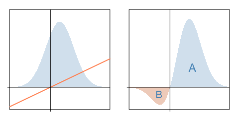
$\text{EU}_0$ is the integral of the curve in the right panel, or the area $A - B$. (This is because $A - B > 0$. Otherwise, we would choose $a = 0$ and have $\text{EU}_0 = 0$.) This is the expected utility of our uninformed decision.

If we can first observe the true value of $\Theta$ before deciding, we can always take the best action for every possible value of $\Theta$. In our example, we will choose $a = 1$ for positive values and $a = 0$ for negative values. In general, the expected utility of the fully informed decision is given by

\[\text{EU}_p = \int_{\theta} \max_{a \in A}\big[u(a,\theta)\big]f_{\Theta}(\theta) d\theta\]

In our example, this is represented by the shaded area:

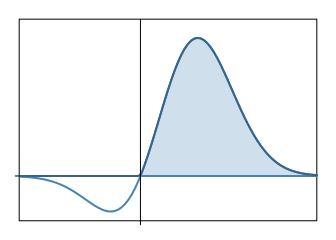
The expected value of perfect information is then $\text{EVPI} = \text{EU}_p - \text{EU}_0$. In our example, we have $\text{EU}_p = A$ and hence $\text{EVPI} = B$.

Imperfect measurements make things a little more complicated. Suppose we can only imperfectly measure $\Theta$ by observing the value of a random variable $X$ that depends on $\Theta$; and then proceed to make an informed decision. Our expected utility is then given by

\[\text{EU}_s = \int_x \max_{a \in A} \bigg[ \int_{\theta} u(a,\theta)f_{\Theta | X}(\theta | x) d\theta \bigg] f_X (x) dx\]

By Bayes’ theorem, we expand the posterior:

\[f_{\Theta | X}(\theta | x) = \frac{f_{\Theta}(\theta) f_{X | \Theta}(x | \theta)}{f_X (x)}\]

Plugging this into the expression for $\text{EU}_s$, the $f_X (x)$ terms cancel and we get

\[\text{EU}_s = \int_x \max_{a \in A} \bigg[ \int_{\theta} u(a,\theta)f_{\Theta}(\theta) f_{X | \Theta}(x | \theta) d\theta \bigg] dx\]

The expected value of sample information is then $\text{EVSI} = \text{EU}_s - \text{EU}_0$.

We’ll use Monte Carlo simulation to approximate $\text{EU}s$. The inner integral is just the expectation of \(u(a,\Theta)f{X

\Theta}(x

\Theta)\). So, for any given action $a$ and observation $x$, we can approximate this integral by simulating lots of random numbers from the distribution of $\Theta$, evaluating this function each time, and then taking the average. We do this for all actions $a$ and then keep the maximum value. This procedure approximates a function $g(x)$, whose integral is $\text{EU}_s$. We then approximate the integral by approximating $g(x)$ for a comb of plausible values of $X$, taking the average, and multiplying by the range (this is basically a Riemann sum approximation except that the integrand isn’t precisely computed).

Note that so far we’ve said nothing about sample size. Sample size will enter into the conditional density \(f_{X

\Theta}(x

\theta)\). If we go through the process above for a range of possible sample sizes, we’ll end up with an idea of how sample size affects the value of information.

A concrete example in R

Let’s consider an example similar to our illustration. We still face a discrete choice between taking some action ($a=1$) and not doing anything ($a=0$). The proposed action has an up-front cost of $1000 and its payoff (in thousands of dollars) is a random variable $\Theta_1$. Doing nothing gives a $0 payoff. (Let’s assume that our utility is linear in dollars.) We have the option of making independent noisy measurements $X_i \sim {iid} \hspace{2 mm} \mathcal{N}(\Theta_1, \Theta_2)$, where $\Theta_2$ represents the variance (noise) of each measurement. (Note the assumption that measurement error is normally distributed. More on this later.) If we know the value of $\Theta_1$, we’ll take action if $\Theta_1 > 1$ and otherwise do nothing. If we’re uncertain about $\Theta_1$ and can’t get more information, we take action if and only if our expected value of $\Theta_1$ exceeds 1.

Let’s assume that our prior probabilities are such that $\Theta_1 \sim \mathcal{N}(0,2^2)$ and $\Theta_2 \sim \mathcal{N}(36,3^2)$, and that $\Theta_1$ and $\Theta_2$ are independent:

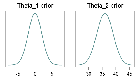
(Strictly speaking, since the variance $\Theta_2$ can’t be negative, we would have to truncate the distribution at zero, or use a distribution with positive support like the gamma distribution. But in our case negative values are so unlikely that this won’t be a problem.)

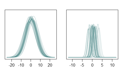
Conditional on $\Theta_1$ and $\Theta_2$, the sample mean of $n$ independent observations is normally distributed with mean $\Theta_1$ and variance $\Theta_2/n$. This gives us the conditional density for the sample mean:

\[f_{X | \Theta_1,\Theta_2}(x | \theta_1, \theta_2) = \sqrt{\frac{n}{2\pi\theta_2}}\exp\Big\{-\frac{n(x-\theta_1)^2}{2\theta_2}\Big\}\]

To get a sense of what these priors look like, I generated 30 realizations of $\Theta_1$ and $\Theta_2$. The plots below show the corresponding sampling densities for individual observations (left) and for sample means with n = 50 (right):

We now have all the input we need for a VOI analysis. Let’s put it into R:

actions = c(0,1)

# hyperparameters
mu_theta1 = 0
sigma_theta1 = 2
mu_theta2 = 36
sigma_theta2 = 3

# random number generators for theta[1,2]
rtheta1 = function(n) rnorm(n, mu_theta1, sigma_theta1)
rtheta2 = function(n) rnorm(n, mu_theta2, sigma_theta2)

# utility function
u = function(actions, theta1){
  # actions: action set
  # theta1:  vector of theta1 realizations
  # returns a matrix of dimension length(theta1) x length(actions)
  sapply(actions, function(a) a * 1000 * (theta1 - 1))
}

# "likelihood" / conditional density of sample mean
xdens = function(x, theta1, theta2, n){
  # x: value of sample mean
  # theta[1,2]: vector of theta[1,2] realizations
  # n: sample size
  dnorm(x, theta1, sqrt(theta2/n))
}

We start by computing $\text{EU}_0$, the expected utility of an uninformed decision:

# preliminaries
set.seed(678)
setpar = function() par(mar=c(3,3,2,1), mgp=c(2,.7,0), las=1)

nsim = 20000 # number of scenarios to simulate
thetas1 = rtheta1(nsim)
U = u(actions, thetas1)
EU = apply(U, 2, mean)
maxEU0 = max(EU) # expected utility of best uninformed action
argmaxEU0 = actions[EU == max(EU)] # best uninformed action

paste("Best action: ", argmaxEU0, "; expected utility: ", maxEU0, sep="")

## [1] "Best action: 0; expected utility: 0"

Without further information, our expected value of $\Theta_1$ is 0, so it’s best to do nothing, for a $0 payoff. We proceed to compute $\text{EU}_s$ for a range of sample sizes by the procedure described above:

ns = c(5, 10, 20, 30, 40, 60, 100, 200)
# sample sizes to consider
xs = seq(-10, 10, by = 0.1)
# comb of plausible values of the sample mean

nsim = 20000 # number of scenarios to simulate
thetas1 = rtheta1(nsim)
thetas2 = rtheta2(nsim)
maxEU1 = rep(0, length(ns))

for (i in 1:length(ns)){
  gs = rep(0, length(xs)) # g(x) values
  for (j in 1:length(xs)){
    likelihoods = xdens(xs[j], thetas1, thetas2, ns[i])
    utilities = u(actions, thetas1)
    prod = likelihoods * utilities
    Eprod = apply(prod, 2, mean)
    gs[j] = max(Eprod)
  }
  maxEU1[i] = mean(gs) * diff(range(xs)) # approx. integral
}

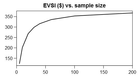
EVSI = maxEU1 - maxEU0 # expected value of sample information

setpar()
plot(ns, EVSI, type="l", lwd=2, main="EVSI ($) vs. sample size", 
     xlim=c(0,200), xaxs="i", xlab="", ylab="")

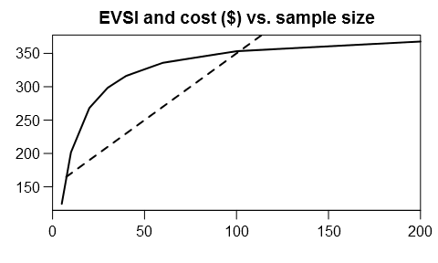
To obtain the optimal sample size, we’ll need a cost function for the measurement. For illustration, let’s assume a fixed cost of $150 and a constant marginal cost of $2 per observation:

cost = function(n) 150 + 2*n

setpar()
plot(ns, EVSI, type="l", lwd=2, main="EVSI and cost ($) vs. sample size",
     xlim=c(0,200), xaxs="i", xlab="", ylab="")
curve(cost(x), lwd=2, lty=2, add=TRUE)

We want to maximize value of information net of experiment cost:

setpar()
plot(ns, EVSI - cost(ns), type="l", lwd=2,
     main="Net payoff ($) vs. sample size",
     xlim=c(0,200), xaxs="i", xlab="", ylab="")
abline(h=0)

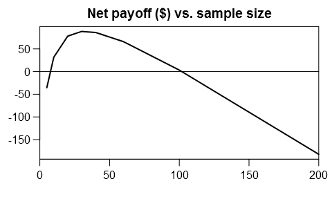
nopt = ns[EVSI - cost(ns) == max(EVSI - cost(ns))]
paste("Optimal sample size: ", nopt, "; Net benefit: ",
      round(max(EVSI - cost(ns))))

## [1] "Optimal sample size:  30 ; Net benefit:  88"

So the optimal sample size is about 30. You need to spend $210 on the experiment, and expect to gain about $298 on average.

Discussion

Recall that we made the assumption that each observation $X_i$ is normally distributed. This is often not the case. (For example, the observations might only take on a few discrete values.) Still, the central limit theorem tells us that for large enough samples, the sample mean $X$ is approximately normal even if the invididual observations aren’t. For many realistic measurements, the approximation is pretty good even with a moderate sample size.

Messier problems might be handled by defining the appropriate conditional density \(f_{X

\Theta_1,\Theta_2}\), or else by directly simulating random samples from the population (this would be more involved than my approach here).

What about the more common experimental scenario of comparing a treatment/intervention group to a control group, to estimate the treatment effect? We model this as taking samples from two populations to estimate the difference between the population means. We can apply the above R code to this question, with minor modifications. In the easiest case, each population is normally distributed with common variance $\Theta_2$. We now let $\Theta_1$ denote the unknown difference between population means, and $X$ will be the observed difference between sample means. If we make $n$ observations of each population, then $X$ is normal with mean $\Theta_1$ and variance $2\Theta_2/n$, and the following is our new conditional density function:

xdens = function(x, theta1, theta2, n){
  dnorm(x, theta1, sqrt(2*theta2/n))
}

The rest of the procedure should be essentially unchanged.

Finally, to apply any of this to practical decision problems, you need to a define reasonable utility function and a reasonable measurement cost function that includes your explicit and implicit costs of running an experiment. At a minimum, you’ll need to monetize subjective benefits and costs (such as your time). You will probably also need to discount future benefits and costs. If it looks like a long experiment is optimal, considering taking into account the cost of delaying your action, maybe by adding $n$ as an argument to the utility function. If you don’t have a clue about how noisy your measurements are going to be, some baseline measurements are probably a good idea before you plan large experiments. And so on. For practical insights applied to self-experiments, I highly recommend gwern’s writeups (see here, here, here, and here).